Note: All charts below were created with Matplotlib and Seaborn.
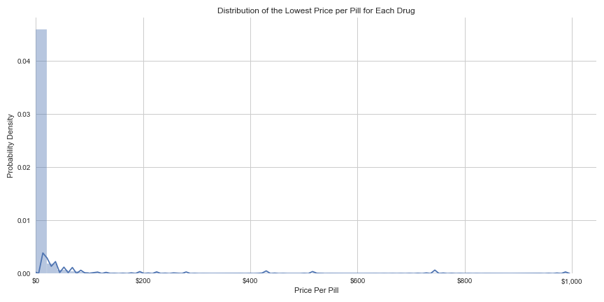
For my second project as a student at Metis, I used linear regression to predict the prices of prescription medications. Focusing only on drugs in pill form, my model contained 1,027 different drugs, and aimed to predict the price per pill for purchasing each medication in the United States. The mean price per pill for the sample of drugs in my model was $15.43, with a standard deviation of $77.25, a distribution so skewed to the right it suggests that these prices become negative on the low-end of the curve. While 97.5% of my sample had a cost per pill of less than $100, the outliers in the dataset were nearly $1,000 per pill. I hoped to gain insight into the factors that determine this great disparity in prescription drug prices, an issue so many Americans face while seeking medical treatment.
I included 18 total features in my linear regression model. Some defined the drug’s chemical properties like molecular weight chemical state, and targeted receptors, while others conveyed its degree of establishment, like the number of manufacturers, patents, clinical trials and dosage forms. I also included the NADAC (National Average Drug Acquisition Cost) for each drug, provided by Medicaid.gov, which was the only feature in the same units as my dependent variable (cost per pill).
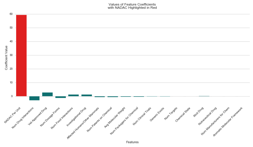
After running my regression, I was excited to see a high R² score of 0.88, and began working on my presentation, confident that my model had uncovered important trends in drug pricing that I could share with my peers. The NADAC not surprisingly had the largest coefficient of all features predicting the cost per pill for a given prescription. It’s magnitude was 59.27, with the second highest being the Number of Drug Interactions at a much lower magnitude of 3.07. I expected this result, since the more a pharmacy has to pay for a particular drug, the more the patient will have to pay in return. However, I hoped my presentation would mostly highlight the other 17 important features I used to predict the price per pill for prescription medications.
To give the other 17 features credibility in making this prediction on their own, I ran my regression without the NADAC and ruefully interpreted the results. Without including the NADAC in the model, my R² score had dropped from 0.88 to 0.04. So I ran a new regression, this time only including one feature–the NADAC, hoping for a score that couldn’t possibly match my original feat of 0.88. To my dismay, this simple linear regression containing only one feature, returned with an R² of 0.91. I woefully began to accept that NADAC was the reason for my original model’s success.
But I need to be sure. Faced with a dilemma, and with my presentation only a few hours away, there were two questions I needed to answer confidently before interpreting my results: Was the NADAC the true reason for my original model’s success? And if not, what could I learn from the other 17 features in my original model?
My answers lied within the VIF (Variance Inflation Factor) of my original model. VIF provides a value for the amount of variance explained by a particular feature in a model. Rather than interpreting the coefficients of the features, which do not indicate the degree to which a given feature is improving model accuracy, the VIF of a given feature offers assurance for how well that feature is explaining the variance of the dataset as a whole. I decided to use VIF to check for how much of the variance in my model was explained by NADAC compared to my other features, hoping that this calculation would allow me to conclude whether the other 17 features had helped in generating my original model’s R² score of 0.88.
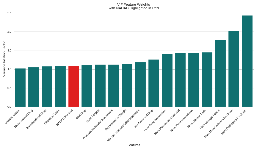
Again, my results surprised me. Though NADAC had the largest coefficient magnitude in my original model across all features at 59.27, (the second highest was -3.07), it ranked 5 out of 18 for low VIF. The results indicated that four other features did a better job of explaining the variance in my dataset than NADAC. Those features were “Generic Exists,” (whether a generic version of the drug is currently on the market), “Nutraceutical Drug”, (whether the drug is considered nutraceutical), “Investigational Drug”, (whether the drug is considered investigational), and “Chemical State”, (whether the drug’s chemical origin is manufactured in solid or liquid form).
It was misleading of me to initially conclude that NADAC was the my most important feature from interpreting the coefficients of my features. VIF allowed for a better informed model choice, and a more accurate interpretation of my feature weights.